

News
Evgeni Dimitrov is the recipient of the 2026 Mathematics Prize of the Institute of Mathematics and Informatics
The Mathematics Prize of the Institute of Mathematics and Informatics was established in 2014 and is awarded every 2 or 3 years, with the selection process initiated by the Institute’s Scientific Council. The prize consists of a statuette, a certificate, and a monetary award, funded through donations. The recipient of the Prize is determined by an international IMI Prize Committee, consisting of 5 to 7 members who are prominent specialists in mathematics.
The 2026 IMI Mathematics Prize was announced on July 6, 2026, during the opening of the International Conference “Mathematics Days in Sofia 2026”. The award was presented by Prof. Julian Revalski, Chairman of the 2026 Prize Committee.
Evgeni Dimitrov, University of Southern California, USA, receives the IMI Prize for outstanding achievements in mathematics for his groundbreaking work in probability theory. His research helps explain complex random phenomena arising in mathematical models of growing interfaces and random matrices. He is also one of the world leaders in the rapidly developing theory of Gibbsian line ensembles.
Dr. Dimitrov has been working in the Department of Mathematics at the University of Southern California (USC) since 2022. From 2018 to 2022, he worked as an assistant professor at Columbia University. His research interests lie in the fields of probability theory, integrable probability, and mathematical physics. He earned his PhD in Mathematics from the Massachusetts Institute of Technology (MIT) under the supervision of Alexei Borodin (2018). He obtained his Bachelor’s degree from Princeton University in 2013.
He is the recipient of numerous prestigious awards, including:
- Simons Award, Simons Foundation International (2025–2030).
- National Science Foundation Award(2021–2024).
- Minerva Foundation Fellowship, Columbia University (2018–2021).
- Bronze medal at the 49th International Mathematical Olympiad (2008) and a silver medal at the 25th Balkan Mathematical Olympiad (2008).
Dr. Dimitrov has extensive research experience with numerous articles accepted for publication in journals such as Probability Theory and Related Fields, Communications in Mathematical Physics, and Annals of Probability. He supervises PhD students and postdocs at USC and mentors many undergraduate students. He has held various teaching positions at USC, Columbia University, and MIT, teaching courses ranging from mathematical analysis to advanced topics in probability theory and mathematical analysis.
The members of the IMI Prize Committee for 2026 were Julian Revalski, Director of the International Center for Mathematical Sciences–Sofia at the Institute of Mathematics and Informatics at the Bulgarian Academy of Sciences, Bulgaria – Chairman of the Prize Committee; Jean-Pierre Bourguignon, Institut des Hautes Etudes Scientifiques, France; Jaqueline Mesquita, University of Campinas, Brazil; Nikolai Nikolov, Institute of Mathematics and Informatics, Sofia, Bulgaria; and Yuri Tschinkel, Courant Institute, USA, Foreign member of the Bulgarian Academy of Sciences.
 Evgeni Dimitrov is the fifth laureate of the IMI Mathematics Prize. Previous recipients of the Prize are Martin Kassabov, Cornell University in Ithaca, USA (2014), Kiril Datchev, Purdue University, USA (2017), Greta Panova, University of Southern California, USA (2020), and Vesselin Dimitrov, Georgia Institute of Technology, USA (2023).
The presentation of the award and Dr Dimitrov’s public lecture will be announced at a later date.
Mathematics Days in Sofia 2026 Officially Opens
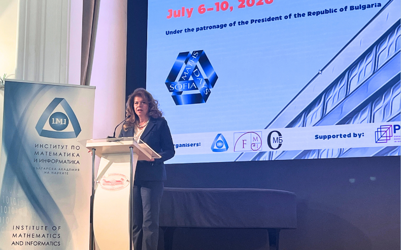
Today, in the “Prof. Marin Drinov” Hall of the Bulgarian Academy of Sciences, the International Conference “Mathematics Days in Sofia” 2026 was officially opened. The event is held under the patronage of the President of the Republic of Bulgaria and is organized by the Institute of Mathematics and Informatics at the Bulgarian Academy of Sciences, jointly with the Faculty of Mathematics and Informatics of Sofia University “St. Kliment Ohridski”, and the Union of Mathematicians in Bulgaria.
The opening of the scientific forum was attended by the President of the Republic of Bulgaria Ms. Iliana Iotova, Prof. Evdokia Pasheva, Vice-President of the Bulgarian Academy of Sciences, Prof. Senya Terzieva-Zhelyazkova, Deputy Minister of Education and Science, Prof. Parvan Parvanov, Rector of Sofia University “St. Kliment Ohridski”, and Prof. Maya Stoyanova, Dean of the Faculty of Mathematics and Informatics at Sofia University. The official opening was led by Prof. Julian Revalski, Chairman of the Program Committee of the conference, President of the Union of Mathematicians in Bulgaria, and Director of the International Center for Mathematical Sciences at IMI-BAS.
Congratulatory addresses to the organizers of the prestigious event were sent by the President of the National Assembly of the Republic of Bulgaria and the Rector of Sofia University “St. Kliment Ohridski”. On behalf of the President of the Bulgarian Academy of Sciences, a greeting was delivered by Prof. Evdokia Pasheva.
The International Conference “Mathematics Days in Sofia” will continue until July 10, 2026. The forum is held every three years, and today marks the start of its fifth edition. To take part in this traditional meeting of Bulgarian mathematicians, more than 200 scientists from 27 countries arrived in Sofia to present their new results in classical and modern fields of mathematics and computer science.
The achievements of Bulgarian specialists in mathematics and computer science has long been recognized, and today a large number of these scientists successfully pursue their careers in prestigious international universities and research centers. Organizing and hosting scientific events like “Mathematics Days in Sofia” brings closer and strengthens contacts with the Bulgarian mathematical community abroad. By creating an appropriate environment for joint scientific projects and partnerships, the forum stimulates the achievement of key results and the discovery of important answers that find real application in all spheres of human development.
By tradition, during the opening of the conference, the 2026 IMI Mathematics Prize was announced, which is awarded every three years to a Bulgarian mathematician under the age of 40 for high achievements in the field of mathematics. The prize was presented by Academician Julian Revalski, Chairman of the Prize Committee.
 The recipient of the 2026 IMI Mathematics Prize is Dr. Evgeni Dimitrov from the University of Southern California, USA. Dr. Dimitrov receives the IMI Prize for outstanding achievements in mathematics for his groundbreaking work in probability theory. His research helps explain complex random phenomena arising in mathematical models of growing interfaces and random matrices. He is also one of the world leaders in the rapidly developing theory of Gibbsian line ensembles.
The International Conference “ Mathematics Days in Sofia 2026″ is held with the support of the Scientific Program “Enhancing the Research Capacity in Mathematical Sciences” (PIKOM), the Ministry of Education and Science, and the Simons Foundation.
More about the conference, its participants, as well as the program of the event can be found at https://mds.math.bas.bg/


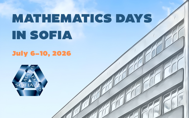
Announcing the 5th International Conference “Mathematics Days in Sofia” (MDS2026)
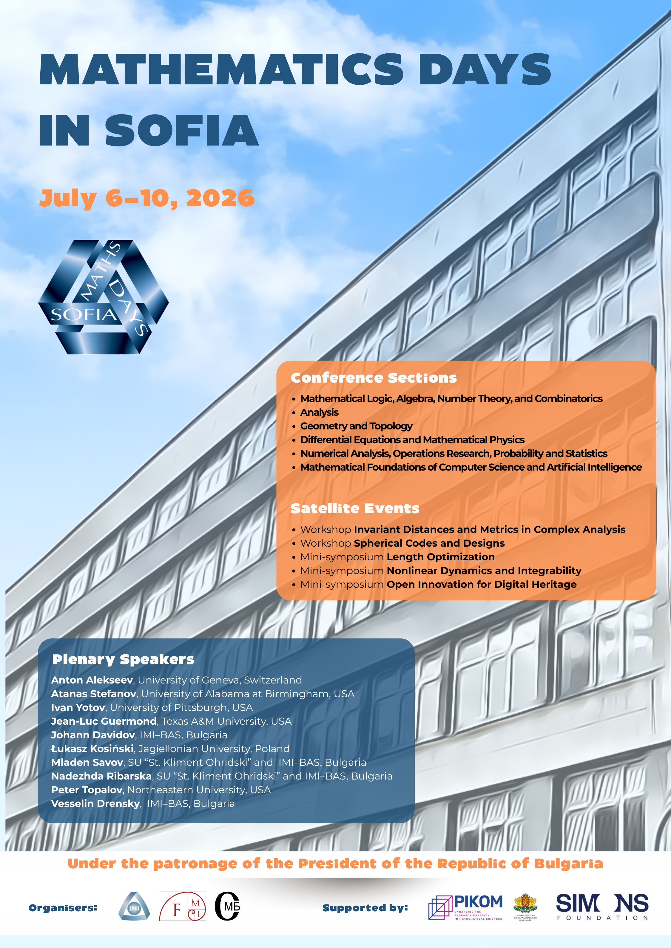 From July 6 to 10, 2026, the Institute of Mathematics and Informatics at the Bulgarian Academy of Sciences (IMI-BAS), in cooperation with the Faculty of Mathematics and Informatics at Sofia University “St. Kliment Ohridski” and the Union of Bulgarian Mathematicians, is organizing the prestigious international conference Mathematics Days in Sofia (MDS2026). The event is held under the patronage of the President of the Republic of Bulgaria.
The fifth edition of this distinguished scientific forum will be officially opened on July 6, 2026, in the “Prof. Marin Drinov” Hall of the Bulgarian Academy of Sciences (Sofia, 1, 15th November Str.), personally by Mrs. Iliana Iotova, President of the Republic of Bulgaria.
The strong traditions of the Bulgarian school of mathematics have been proven over time by the dozens of world-renowned scientists and researchers it has nurtured and established on the global scientific stage. While many of them are successfully developing their careers in prestigious scientific centers around the world, one of our greatest challenges remains retaining young talent and building sustainable bridges with our colleagues abroad. By organizing scientific forums of this scale, we strengthen and deepen ties with the Bulgarian mathematical diaspora and provide participants with opportunities for successful collaborative research.
During the opening ceremony of MDS2026, the IMI Mathematics Prize for 2026 for excellent achievements in mathematics will be awarded. The prize is awarded every three years to a Bulgarian mathematician under the age of 40 for outstanding achievements in mathematics. The award will be introduced by Prof. Julian Revalski, Chairman of the Prize Committee, and will be presented by the President of the Republic of Bulgaria. The previous laureates of the Prize are Martin Kassabov, Cornell University, Ithaca, USA (2014); Kiril Datchev, Purdue University, USA (2017); Greta Panova, University of Southern California, USA (2020); and Vesselin Dimitrov, Georgia Institute of Technology, USA (2023).
Mathematics Days in Sofia has established itself as a key event that brings together leading scientists, researchers, and young colleagues from all over the world to exchange experience, share their latest discoveries, and outline future directions for the development of mathematical sciences and informatics.
More information about the program, speakers, and satellite events of MDS2026 can be found on the official conference website.
The International Conference Mathematics Days in Sofia 2026 is supported by the Scientific Program Enhancing the Research Capacity in Mathematical Sciences (PIKOM), the Ministry of Education and Science, and the Simons Foundation.
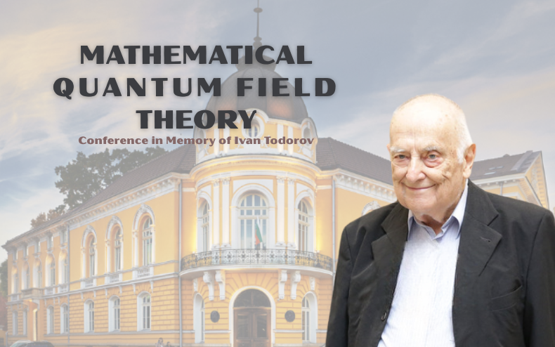
International Conference in Memory of Academician Ivan Todorov
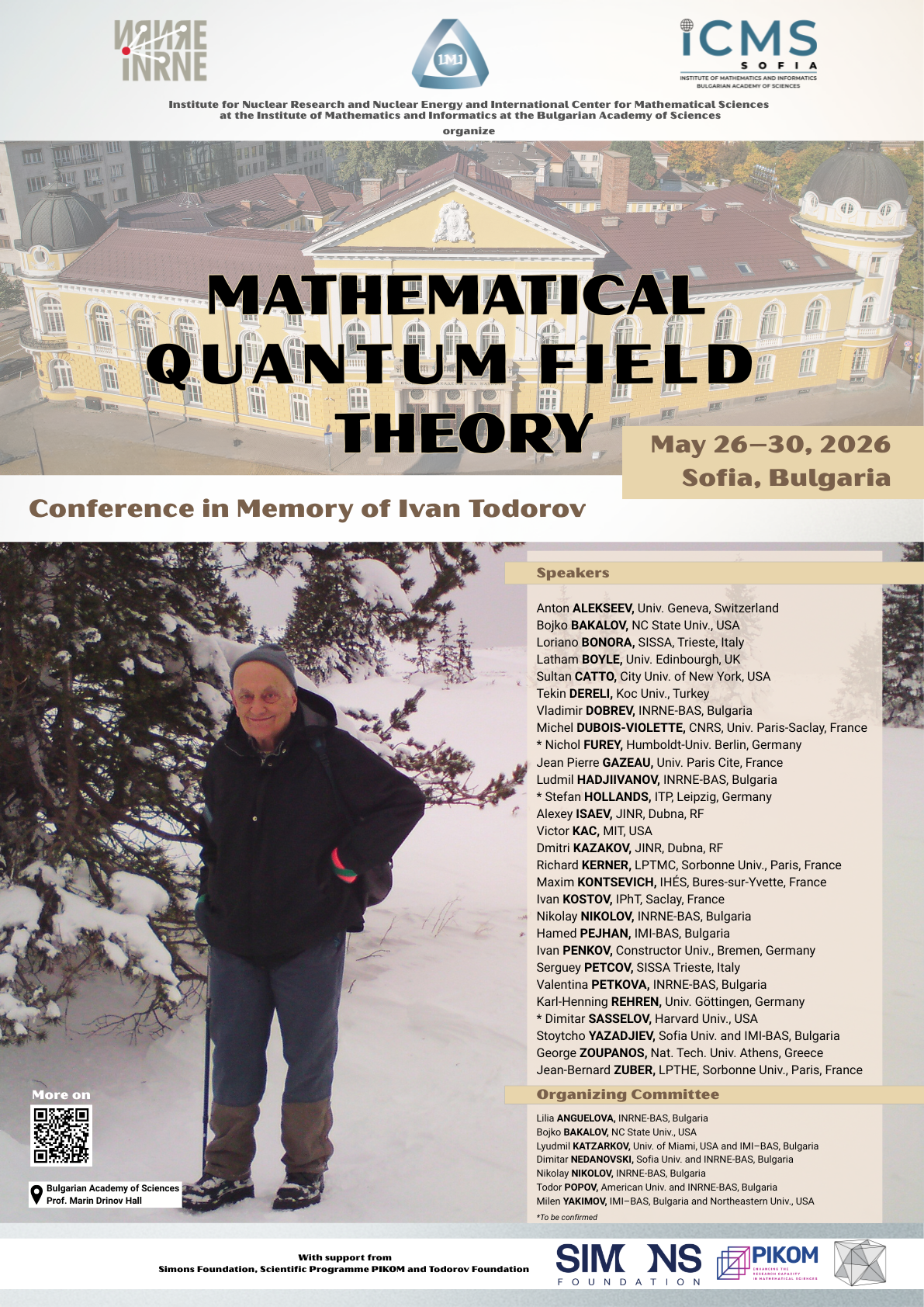 May 26 to May 30, 2026, the Bulgarian Academy of Sciences will host the international conference Mathematical Quantum Field Theory in memory of the renowned Bulgarian theoretical and mathematical physicist, Academician Ivan Todorov, who passed away on February 14, 2025.
Academician Todorov was a scholar with extraordinary achievements and worldwide recognition in the field of modern theoretical physics—particularly in particle theory, high-energy physics, and the mathematical foundations of physics. Throughout his long scientific career, he maintained numerous fruitful collaborations with prominent mathematicians and mathematical physicists from around the world.
The Mathematical Quantum Field Theory conference aims to cover a broad range of topics of broad interest to both physics and mathematics, while also bringing together close collaborators of Academician Todorov and researchers whose work has been significantly influenced by him. Among the speakers are many leading physicists and mathematicians. Academician Todorov had been serving on the advisor board of ICMS from the date it was established.
The conference is organized by the Institute for Nuclear Research and Nuclear Energy – BAS and the International Center for Mathematical Sciences – Sofia (ICMS-Sofia) at the Institute of Mathematics and Informatics, Bulgarian Academy of Sciences with the support from Simons Foundation, Research Program Enhancing the Research Capacity in Mathematical Sciences (PIKOM), and Todorov Foundation.
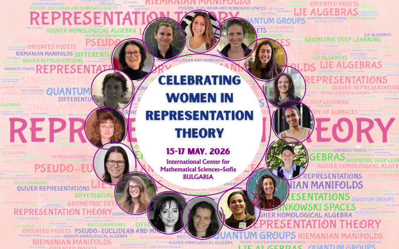
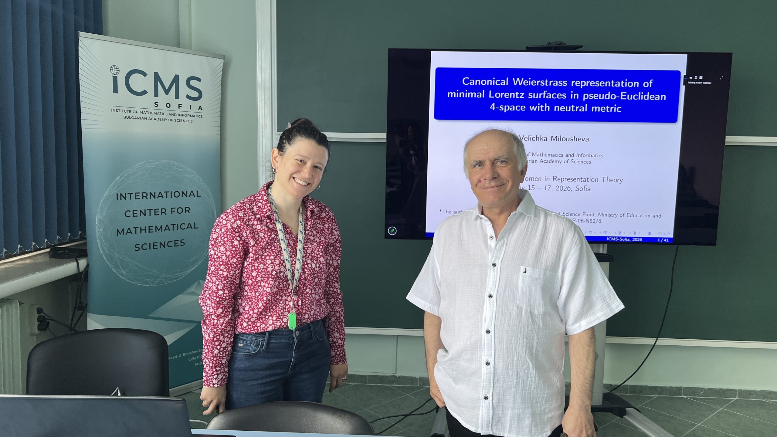
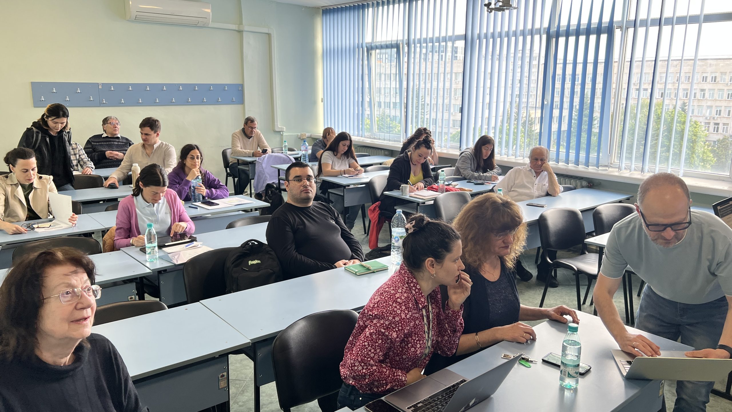
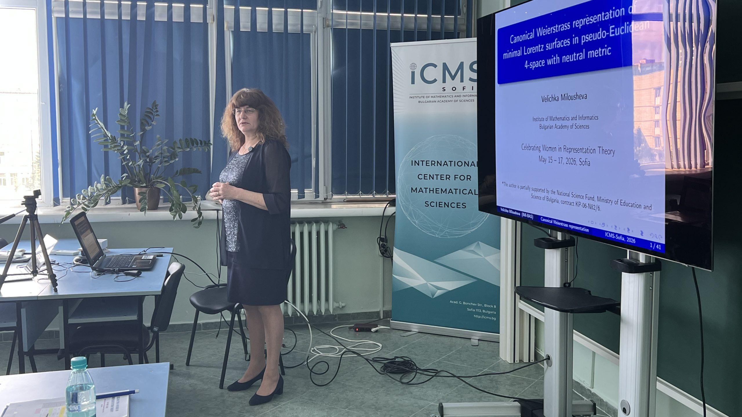
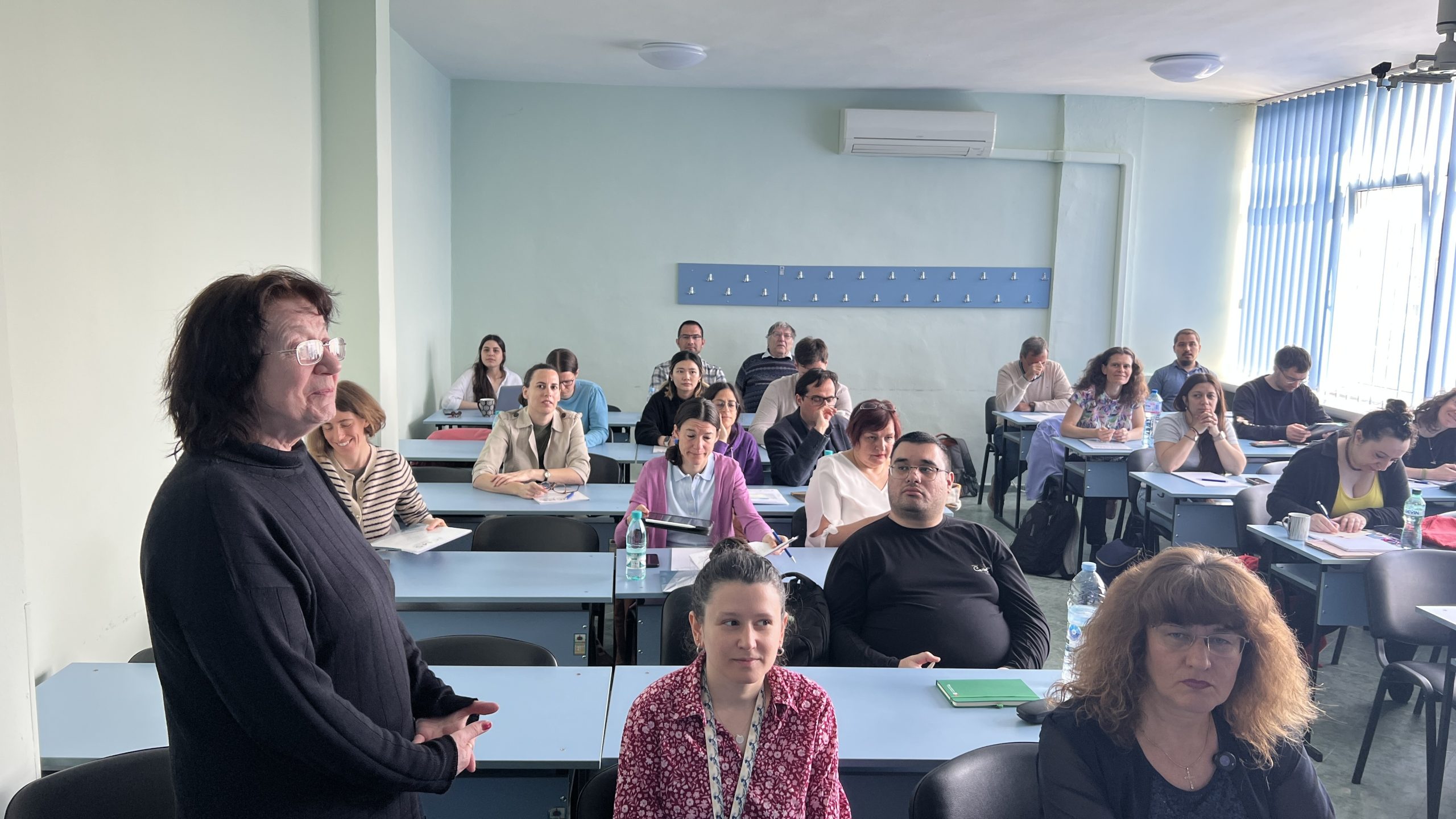
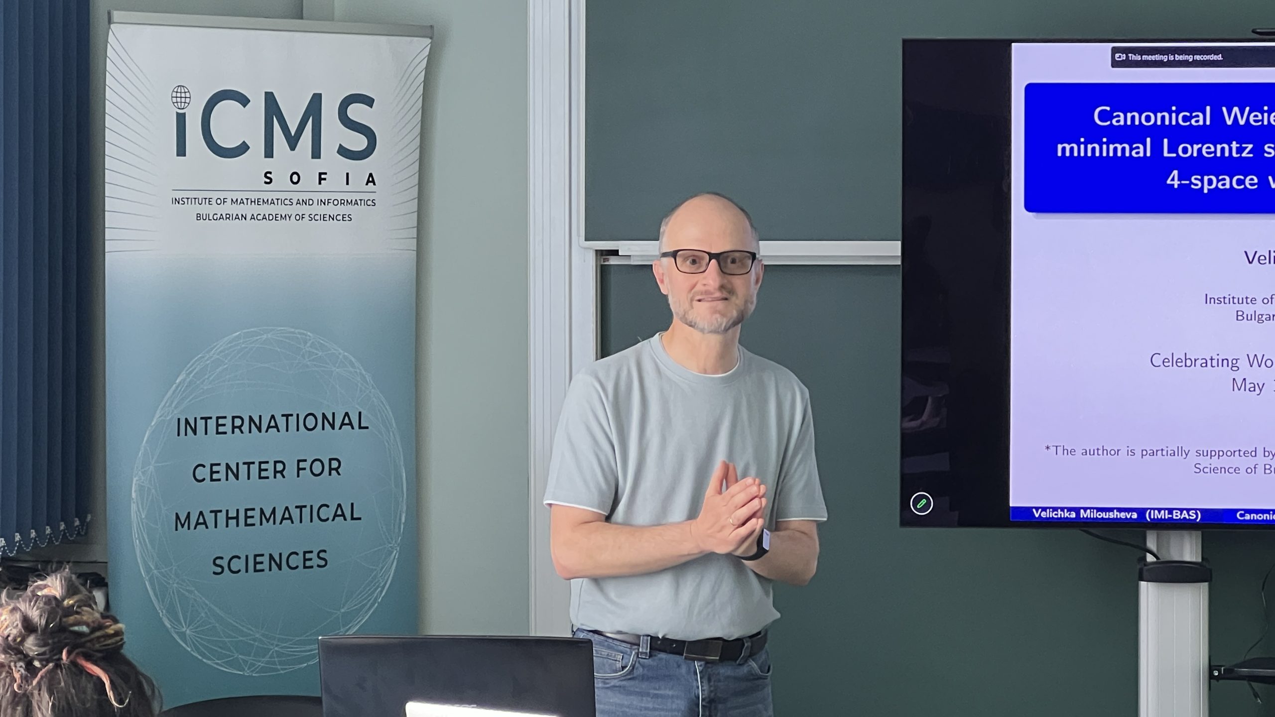
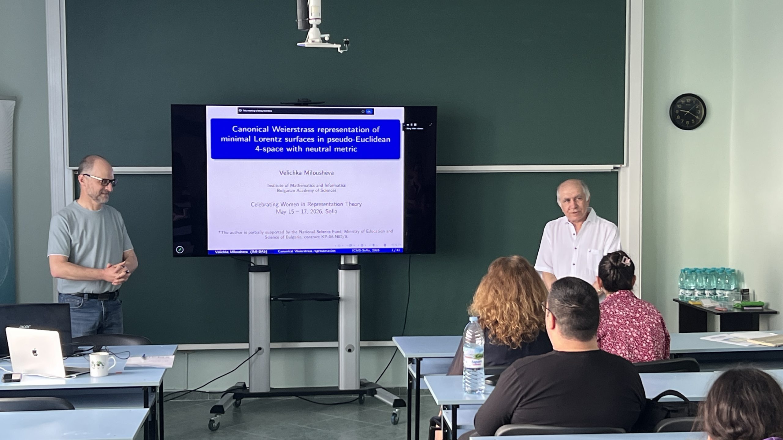
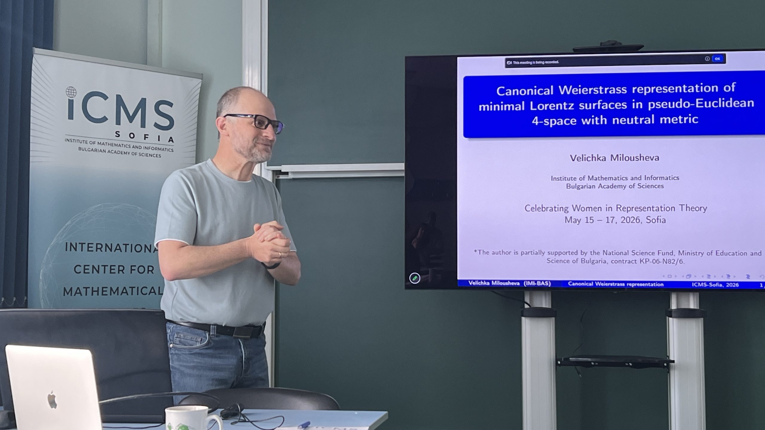
IMI hosts the International Conference “Celebrating Women in Representation Theory”
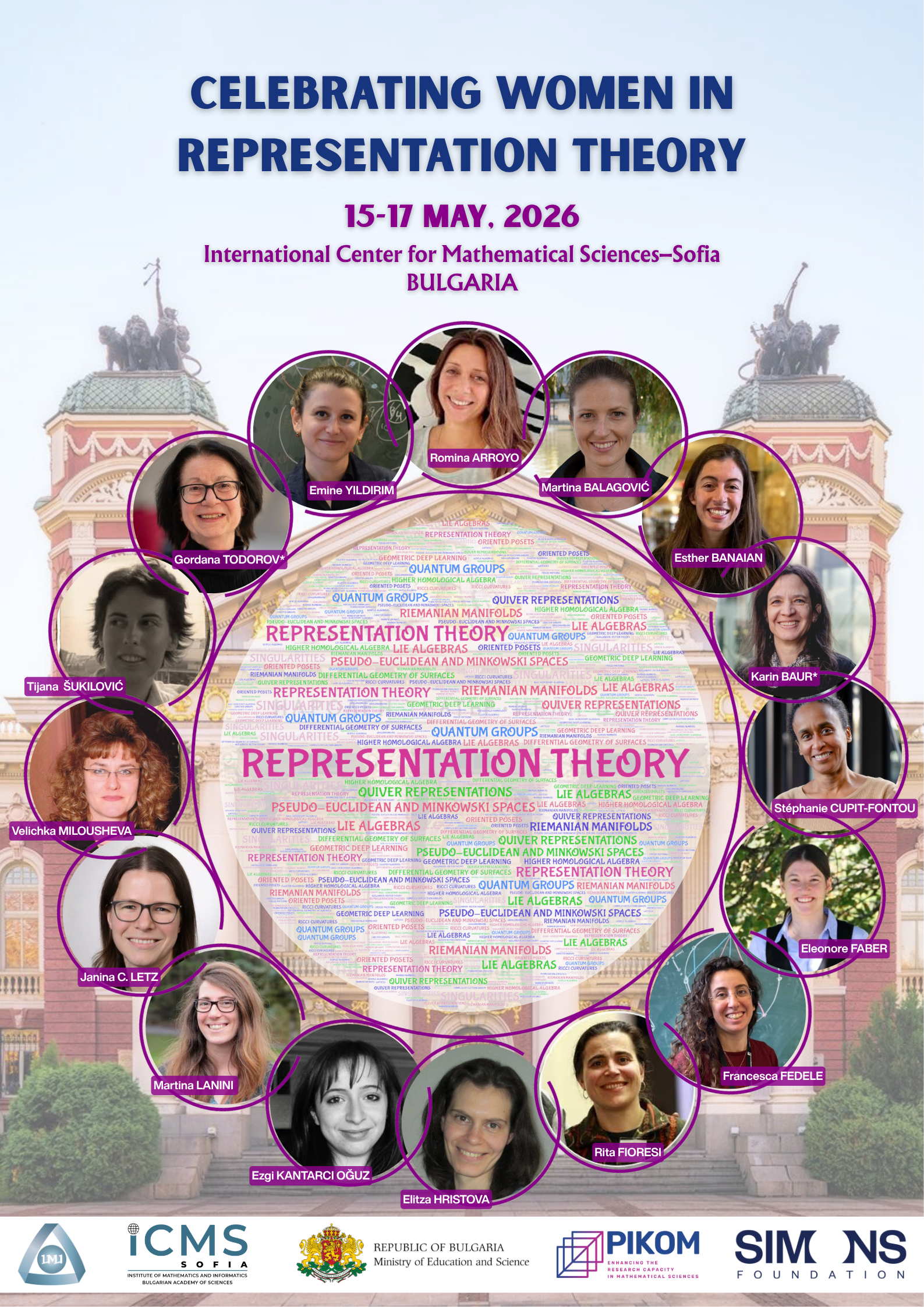 From May 15 to 17, 2026, the International Center for Mathematical Sciences in Sofia (ICMS-Sofia) at the Institute of Mathematics and Informatics is hosting the prestigious international conference Celebrating Women in Representation Theory. The event is part of the activities developed by the Quantum Groups and Cluster Algebras research group at ICMS-Sofia, led by Prof. Milen Yakimov.
The forum was officially opened this morning by Prof. Peter Boyvalenkov, Director of the Institute of Mathematics and Informatics. In his address to the participants, he emphasized the importance of such events for the development the role of IMI as a leading center for international scientific cooperation. A welcoming speech was also delivered by Prof. Velichka Milousheva, Deputy Director of IMI and Deputy Director of ICMS-Sofia. She noted that today’s event is a natural continuation of the Women in Mathematics in South-Eastern Europe initiative—an international conference first held in December 2020, which has since become an annual meeting for female mathematicians from the Balkans and the region.
The conference aims to highlight the contributions of women mathematicians in one of the most dynamic fields of modern algebra. The program includes presentations of the latest scientific results, discussions on current problems, and opportunities for new collaborations in representation theory and adjacent areas. The talks featured in the program cover key topics in modern algebra, group theory, cluster algebras, and quantum groups. Beyond the scientific agenda, the event strives to increase the visibility of women in mathematics and provide support for young scientists in their career development.
Further information regarding the program and speakers can be found on the conference website.
The international conference is organized with the support of the Simons Foundation and the Scientific Program “Enhancing Research Capacity in Mathematical Sciences” (PIKOM).


Administration
IMI PRIZE
IMI MATHEMATICS PRIZE
Please donate
BIC: UNCRBGSF
IBAN: BG32UNCR76303100117336
Address: Institute of Mathematics and Informatics,
Acad. G. Bonchev Str., Block 8,
1113 Sofia
VAT No.: BG000665249


Useful Links