
News
International Conference in Memory of Academician Ivan Todorov
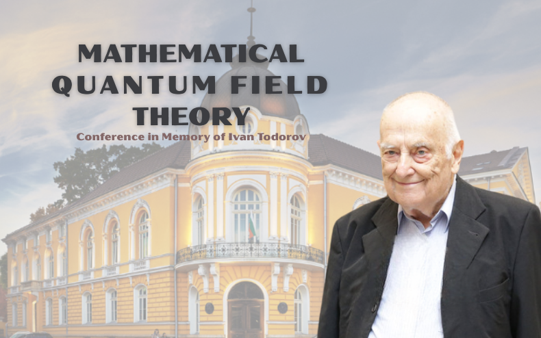
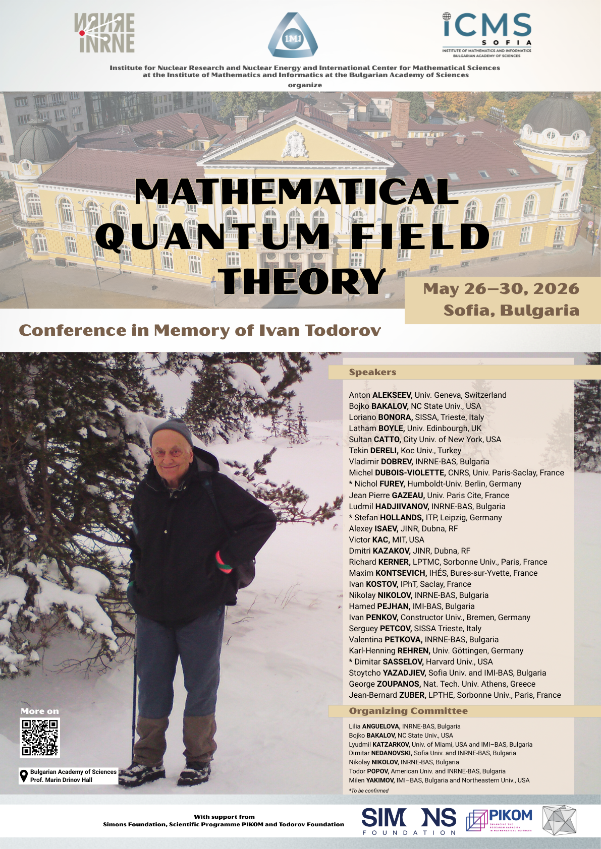 May 26 to May 30, 2026, the Bulgarian Academy of Sciences will host the international conference Mathematical Quantum Field Theory in memory of the renowned Bulgarian theoretical and mathematical physicist, Academician Ivan Todorov, who passed away on February 14, 2025.
Academician Todorov was a scholar with extraordinary achievements and worldwide recognition in the field of modern theoretical physics—particularly in particle theory, high-energy physics, and the mathematical foundations of physics. Throughout his long scientific career, he maintained numerous fruitful collaborations with prominent mathematicians and mathematical physicists from around the world.
The Mathematical Quantum Field Theory conference aims to cover a broad range of topics of broad interest to both physics and mathematics, while also bringing together close collaborators of Academician Todorov and researchers whose work has been significantly influenced by him. Among the speakers are many leading physicists and mathematicians. Academician Todorov had been serving on the advisor board of ICMS from the date it was established.
The conference is organized by the Institute for Nuclear Research and Nuclear Energy – BAS and the International Center for Mathematical Sciences – Sofia (ICMS-Sofia) at the Institute of Mathematics and Informatics, Bulgarian Academy of Sciences with the support from Simons Foundation, Research Program Enhancing the Research Capacity in Mathematical Sciences (PIKOM), and Todorov Foundation.
IMI hosts the International Conference “Celebrating Women in Representation Theory”
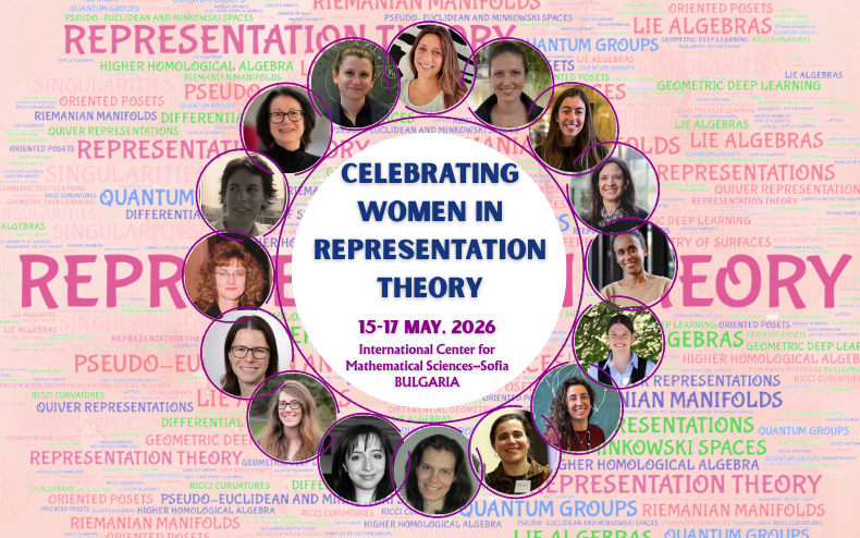
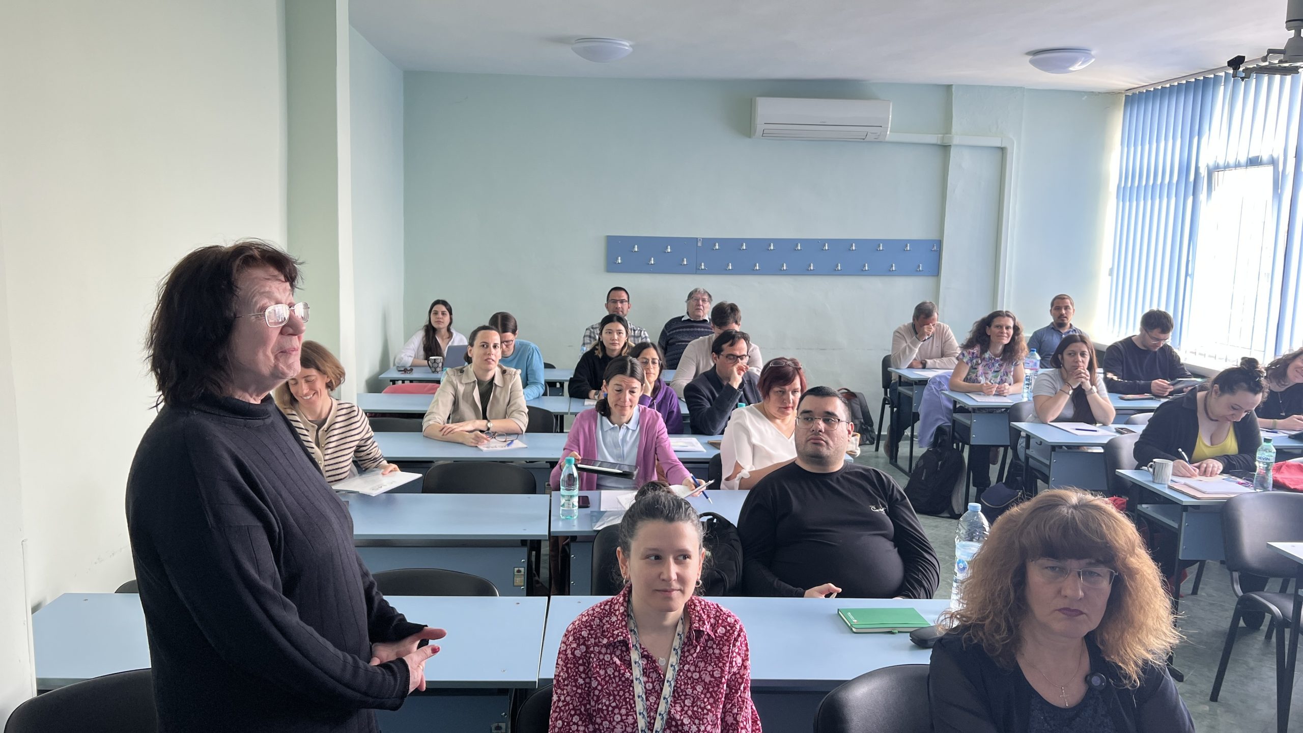
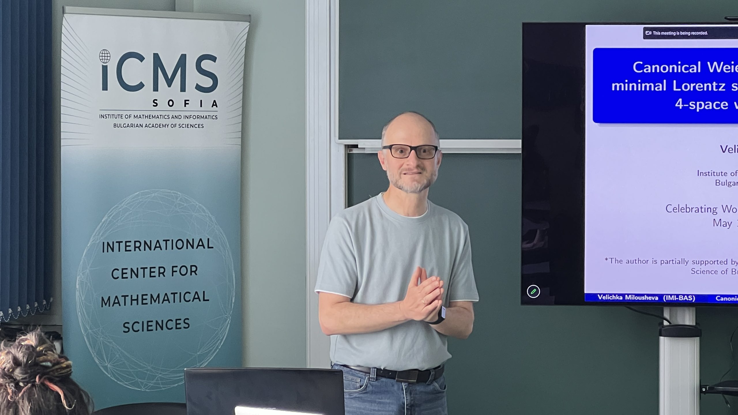
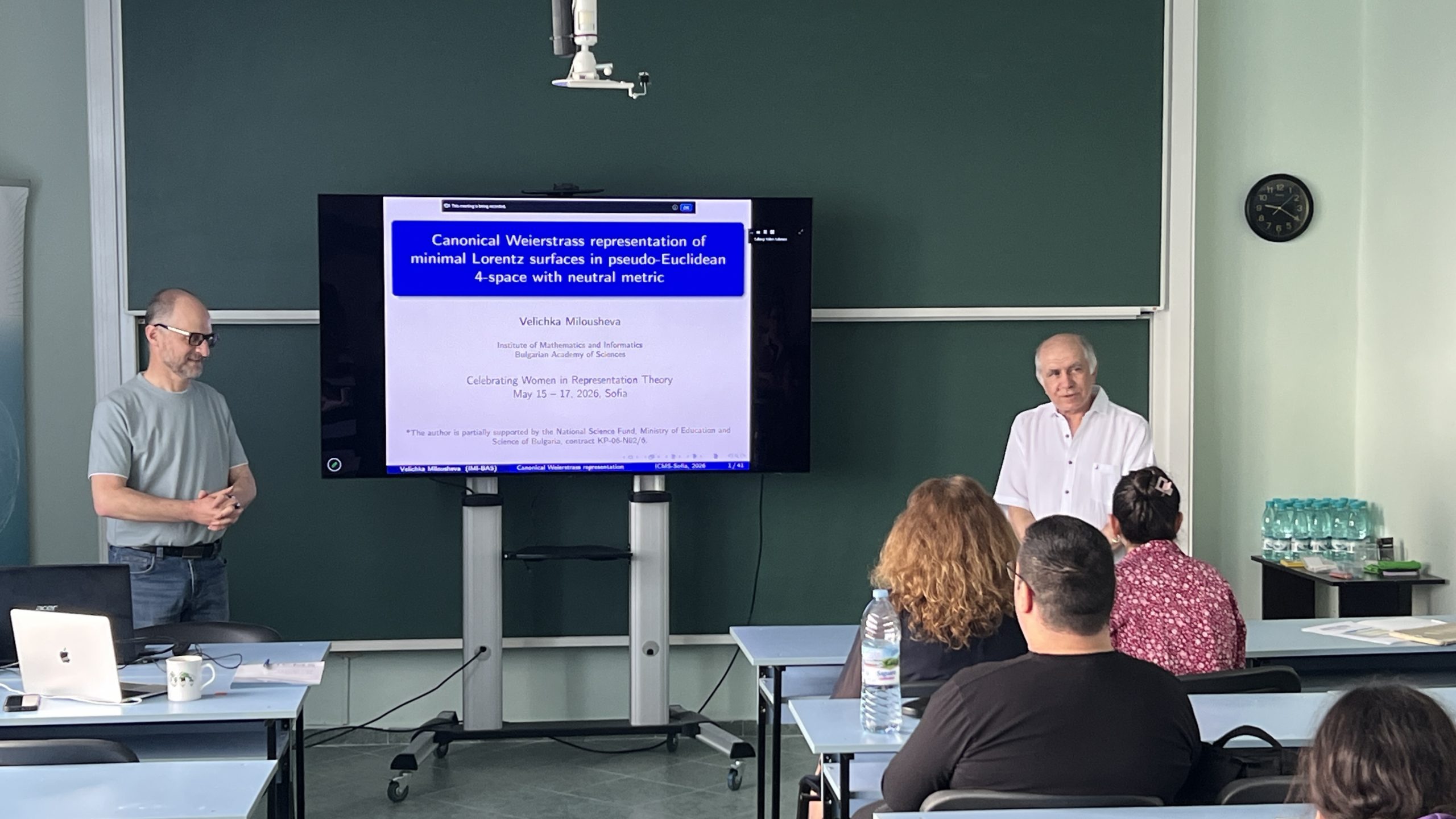
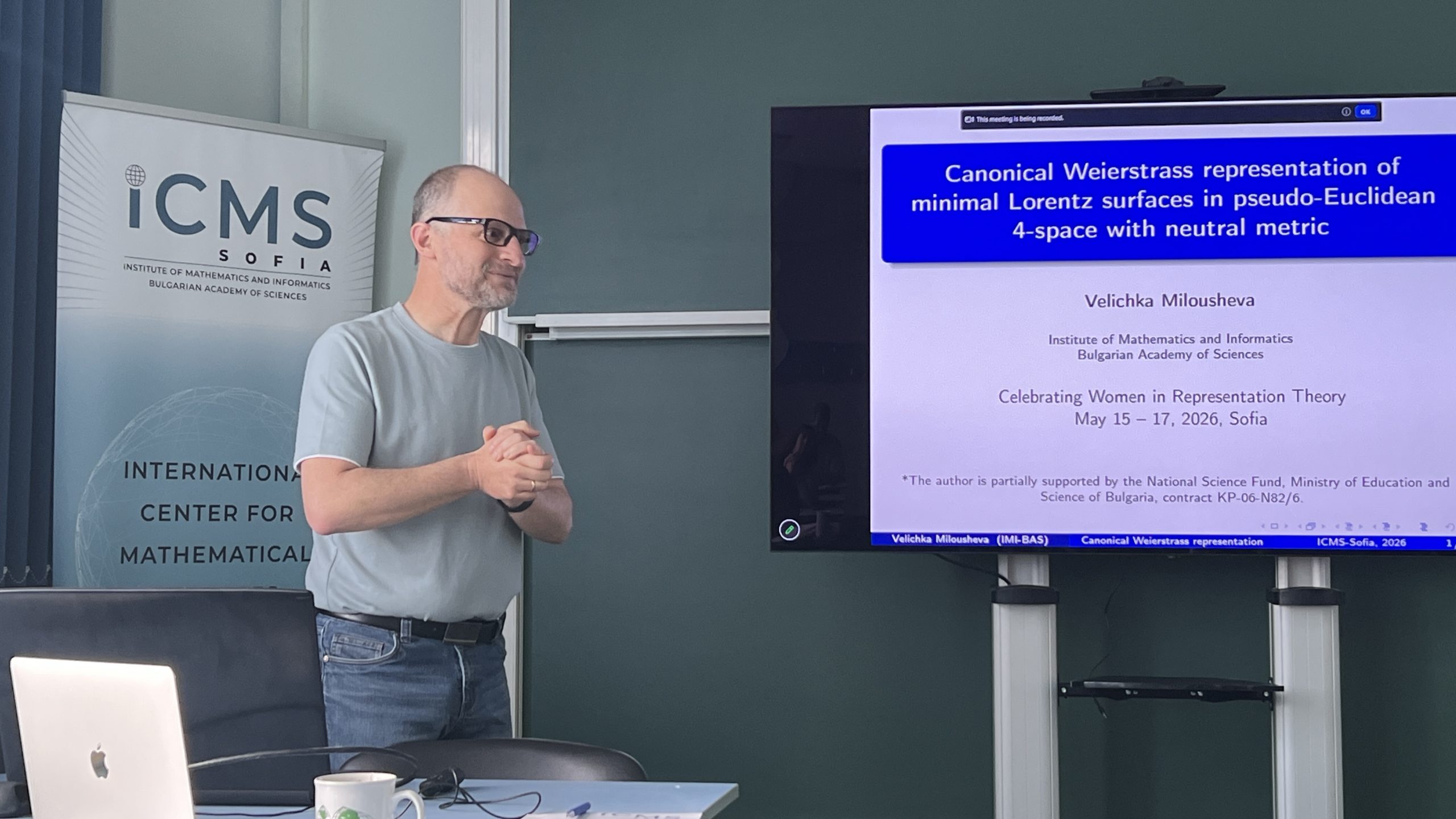
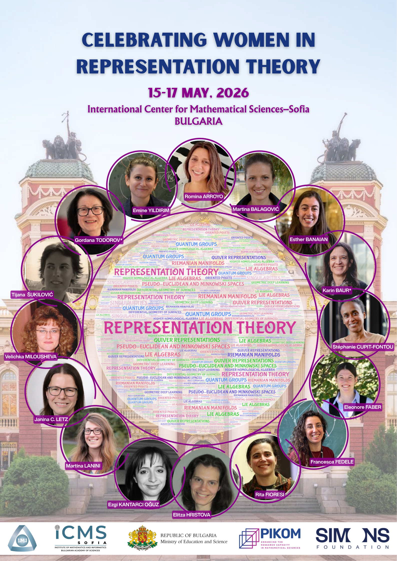 From May 15 to 17, 2026, the International Center for Mathematical Sciences in Sofia (ICMS-Sofia) at the Institute of Mathematics and Informatics is hosting the prestigious international conference Celebrating Women in Representation Theory. The event is part of the activities developed by the Quantum Groups and Cluster Algebras research group at ICMS-Sofia, led by Prof. Milen Yakimov.
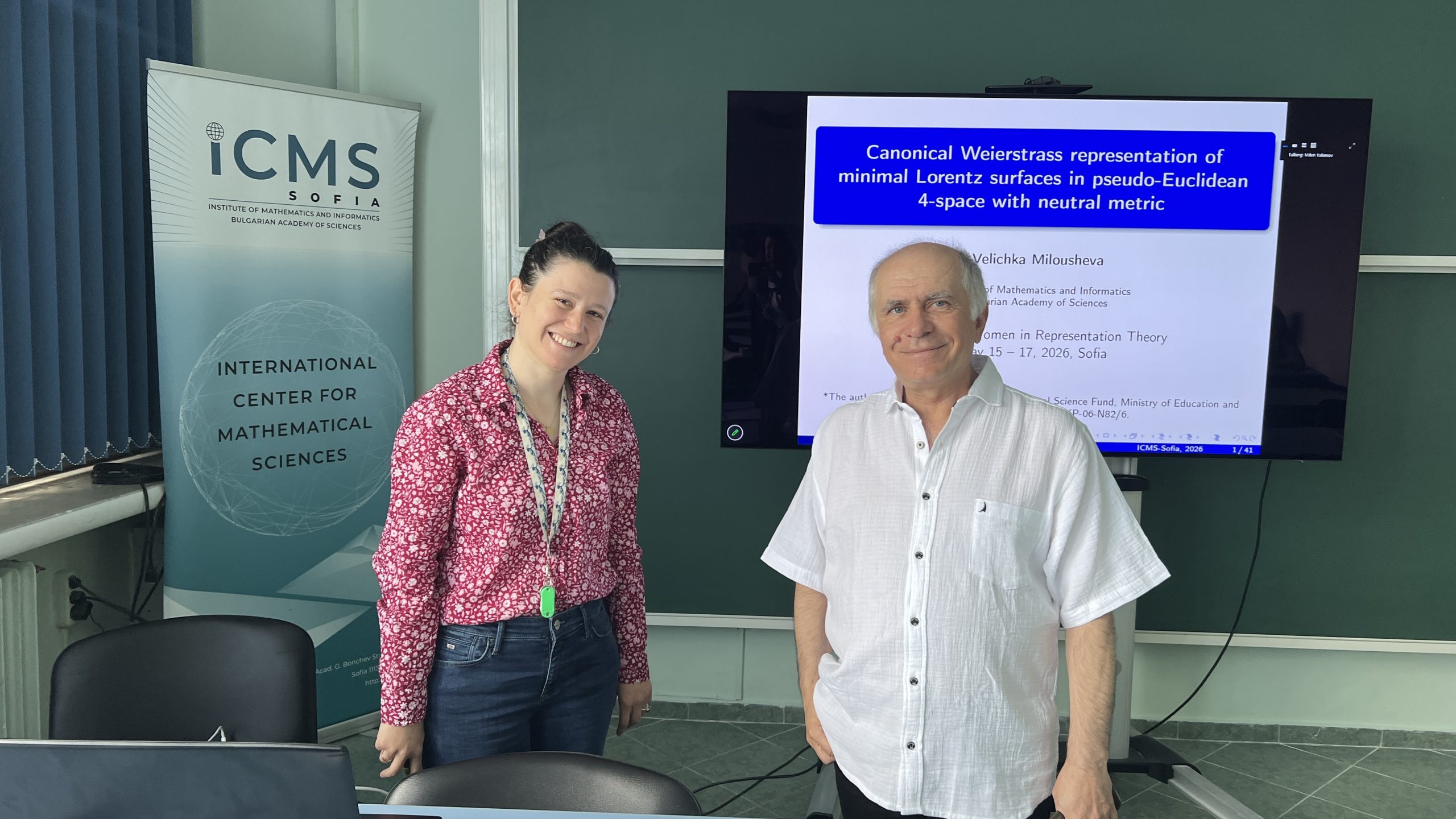
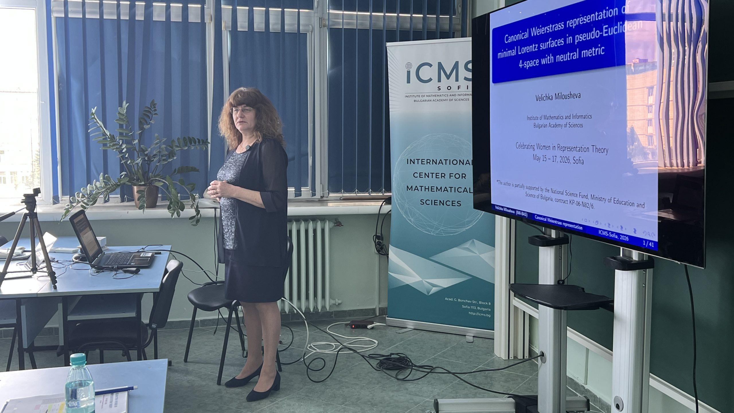
The forum was officially opened this morning by Prof. Peter Boyvalenkov, Director of the Institute of Mathematics and Informatics. In his address to the participants, he emphasized the importance of such events for the development the role of IMI as a leading center for international scientific cooperation. A welcoming speech was also delivered by Prof. Velichka Milousheva, Deputy Director of IMI and Deputy Director of ICMS-Sofia. She noted that today’s event is a natural continuation of the Women in Mathematics in South-Eastern Europe initiative—an international conference first held in December 2020, which has since become an annual meeting for female mathematicians from the Balkans and the region.
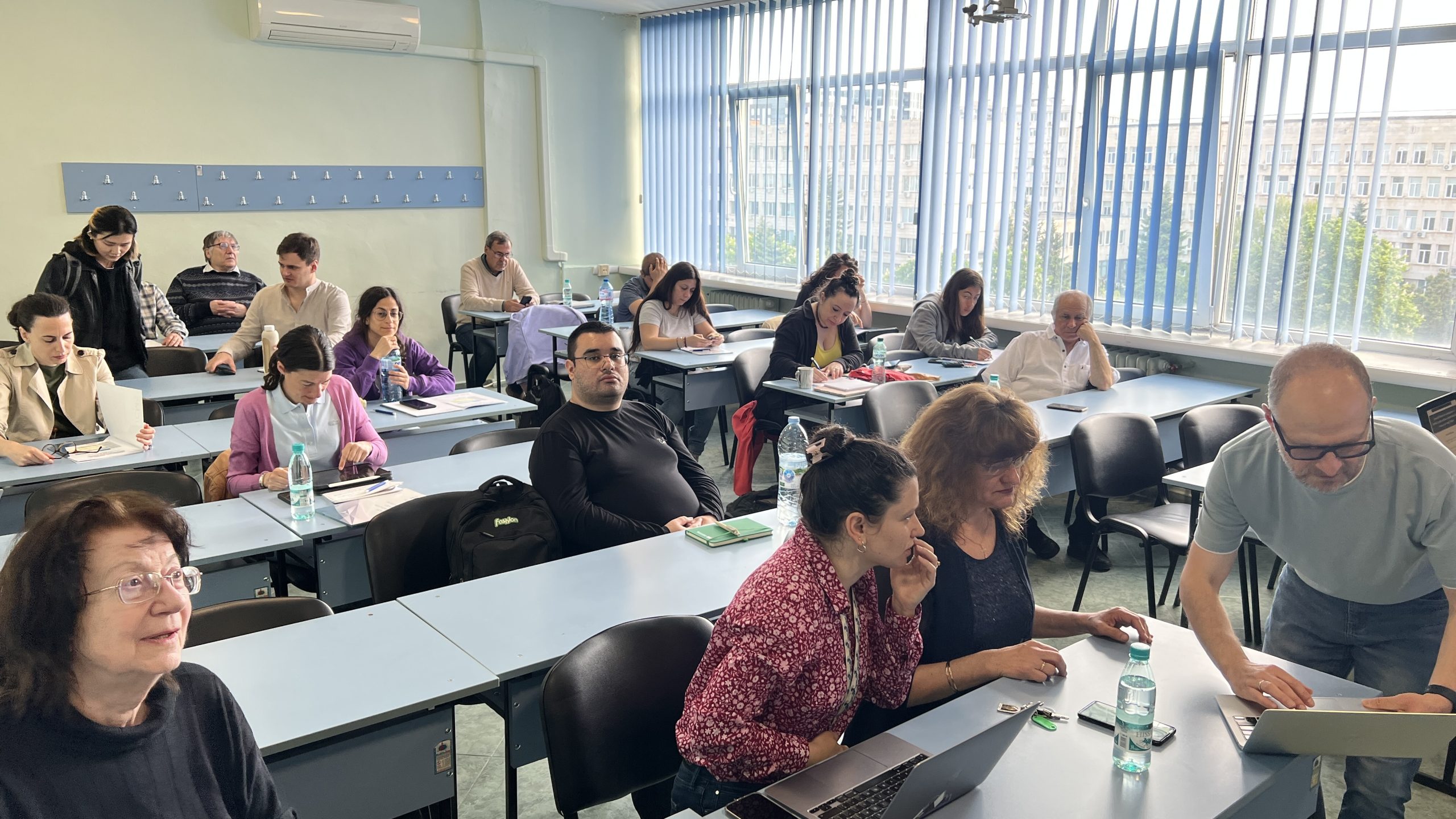
The conference aims to highlight the contributions of women mathematicians in one of the most dynamic fields of modern algebra. The program includes presentations of the latest scientific results, discussions on current problems, and opportunities for new collaborations in representation theory and adjacent areas. The talks featured in the program cover key topics in modern algebra, group theory, cluster algebras, and quantum groups. Beyond the scientific agenda, the event strives to increase the visibility of women in mathematics and provide support for young scientists in their career development.
Further information regarding the program and speakers can be found on the conference website.
The international conference is organized with the support of the Simons Foundation and the Scientific Program “Enhancing Research Capacity in Mathematical Sciences” (PIKOM).


Heart of Agile in the Age of AI – Alistair Cockburn in Sofia
The Institute of Mathematics and Informatics is pleased to announce a public lecture by one of the founding fathers of the Agile movement, Dr. Alistair Cockburn. The event, titled Heart of Agile in the Era of AI, will take place on May 26, 2026, at 19:00 in the Mirror Hall of Sofia University “St. Kliment Ohridski.”
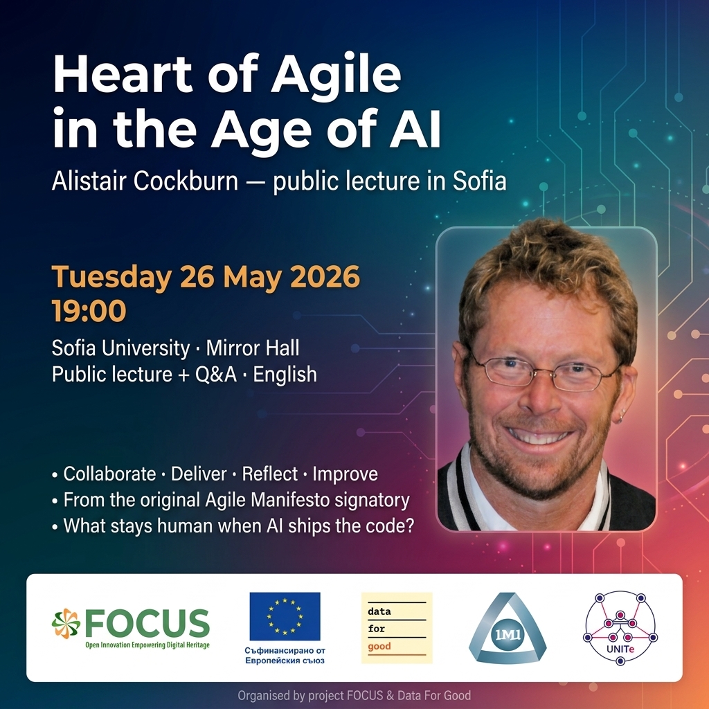 Dr. Cockburn is a world-renowned expert, an original signatory of the Agile Manifesto (2001), and the author of the industry-standard Writing Effective Use Cases. His talk will address the Heart of Agile (Collaborate, Deliver, Reflect, Improve) as a practical compass in a landscape increasingly dominated by AI tools.
His visit is hosted by the Focus: ERA Chair project, implemented at the Institute of Mathematics and Informatics of the Bulgarian Academy of Sciences. The project emphasizes the digitization of cultural heritage — a field where technology meets history and collective memory. FOCUS (Fostering Open Cultural Heritage through Open Innovation and Open Science) operates at this very intersection of technology, culture, and innovation, aiming to transform how we preserve and experience cultural heritage in the digital age. The theme Heart of Agile highlights the importance of collaboration, user value, reflection, and adaptation as the foundation for creating real, effective solutions.
Key Topics:
- Why the four core verbs of Agile are more critical than a list of “values.”
- Slicing ambitious work into small, demonstrable steps.
- AI’s impact: Faster production vs. sharper collaboration challenges.
- Practical lessons from XP and real-world organizations.
The lecture is aimed at developers, architects, product leaders, students, and anyone involved in building creative digital products. As technology accelerates production, the need for clear communication and meaningful feedback grows. Dr. Cockburn will share insights on how to maintain the “human” element of software craft while leveraging modern tools to move fast without “losing the plot.”
Attendance is free of charge, but registration is required via this registration form to secure your spot.
FOCUS Project announces a competition for admission of full-time doctoral students
Institute of Mathematics and Informatics at the Bulgarian Academy of Sciences
announces a competition for admission of full-time doctoral students
under Art. 21, para. 7 of the Higher Education Act,
with an application deadline of 06.06.2026

In implementation of Project BGRFPR002-1.016-0002 “European Chair for the Promotion of Digital Cultural Heritage through Open Innovation and Open Science” (FOCUS), competitions are announced for the admission of full-time doctoral students under Art. 21, para. 7 of the Higher Education Act, in the field of higher education 4. Natural Sciences, Mathematics and Informatics, professional field 4.6. Informatics and Computer Science, doctoral programme “Informatics”, on the topics listed in the table below.
The competition is open to candidates from the country and abroad.
Only candidates who meet the requirements listed below are eligible to participate. They must be enrolled in full-time doctoral studies and, at the time of the announcement of the procedure, must not be registered as doctoral students at any higher education institution or scientific organization. Candidates who have already obtained the educational and scientific degree “Doctor,” as well as those who have been dismissed from a doctoral programme with or without the right to defend, are not eligible.
The admission examinations consist of two parts – one in the specialty and one in a foreign language. The exam syllabus for the specialty examination is available for download at the following links:
Candidates who successfully pass the specialty examination (at least “Very Good” 4.50) and the foreign language examination (at least “Good” 4.00) will be invited to an interview conducted by the Project Management Team.
Approved doctoral candidates will be employed under a labour contract for up to 3 years (for the duration of the doctoral programme) at IMI-BAS, with a full-time workload of 8 hours per day and a salary of €1650. For international doctoral students, an additional €350 is provided. Additional funding is available for travel for conference participation and scientific exchanges up to €2000 per year.
For all other matters related to the admission of doctoral students under this competition, the Regulations for Doctoral Admissions at the Bulgarian Academy of Sciences and national legislation shall apply.
| Doctoral Topic | Proposed by |
| Infrastructures and open solutions for collections as data in Bulgarian cultural heritage institutions | Assoc. Prof. Dr. Milena Dobreva |
| Methods and technologies for integration, semantic enrichment and mapping of open data for public art | Assoc. Prof. Dr. Milena Dobreva |
| 3D modelling of cultural heritage objects: methods for creation, semantic enrichment and valorisation as digital twins | Assoc. Prof. Dr. Vesela Statkova |
From 07.05.2026 to 06.06.2026, candidates shall submit an application form accompanied by the following documents:
- Curriculum Vitae (European format, in Bulgarian)
- Declaration under §5 of the Additional Provisions of Council of Ministers Decree No. 90/26.05.2000 for lack of prior/current full-time doctoral studies
- Master’s degree diploma with its annex. If the diploma has not yet been issued, the candidate must submit an academic transcript showing the average grade from semester examinations with the course workload and the grade from the thesis defence or state examination. A minimum overall grade of “Very Good” (4.50) is required.
- Certificate of recognition of higher education in Bulgaria (issued by a Bulgarian higher education institution or by the National Centre for Information and Documentation – NACID) for persons who obtained their Master’s degree abroad.
Documents are to be submitted to the Human Resources Department (Room 205) of IMI or sent to the email address a.avramova@math.bas.bg.
Contact phone: +359 2 979 3846 – Dr. Aneta Avramova, HR inspector, responsible for academic development.
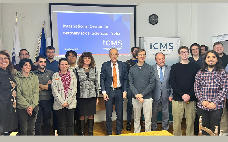
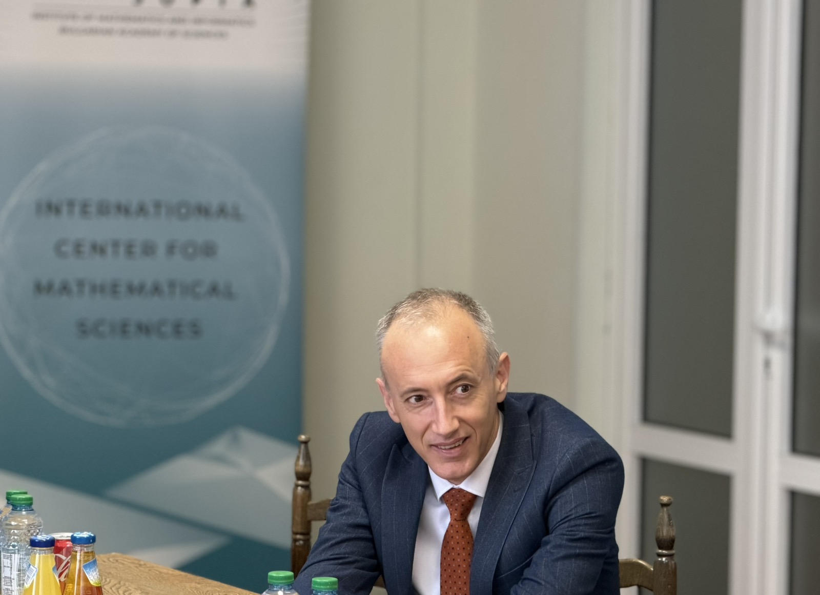
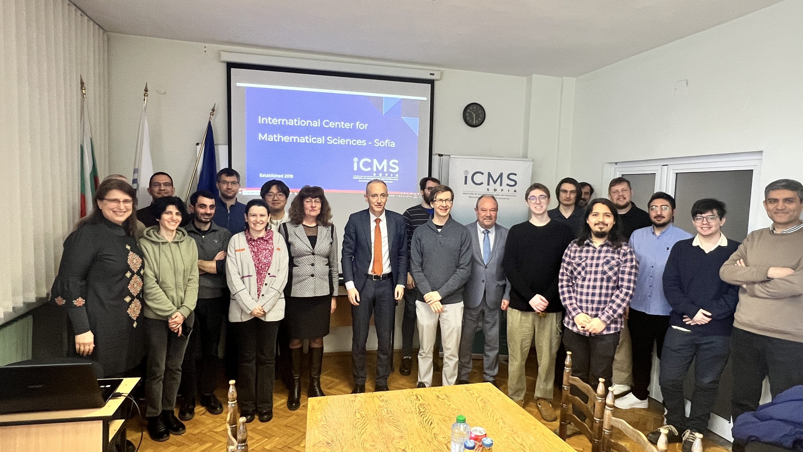
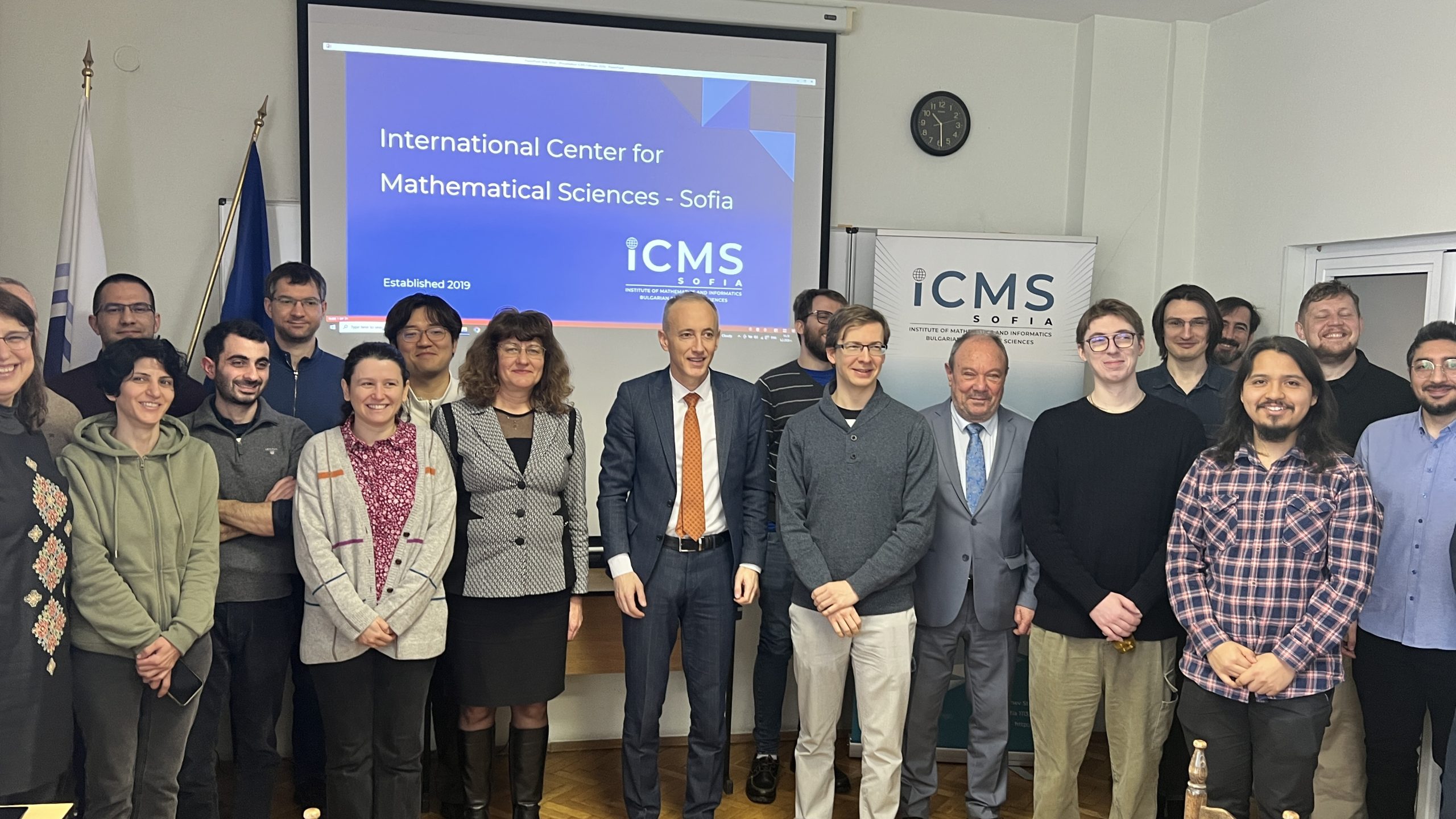
Minister of Education and Science Krasimir Valchev visits the International Center for Mathematical Sciences at IMI-BAS
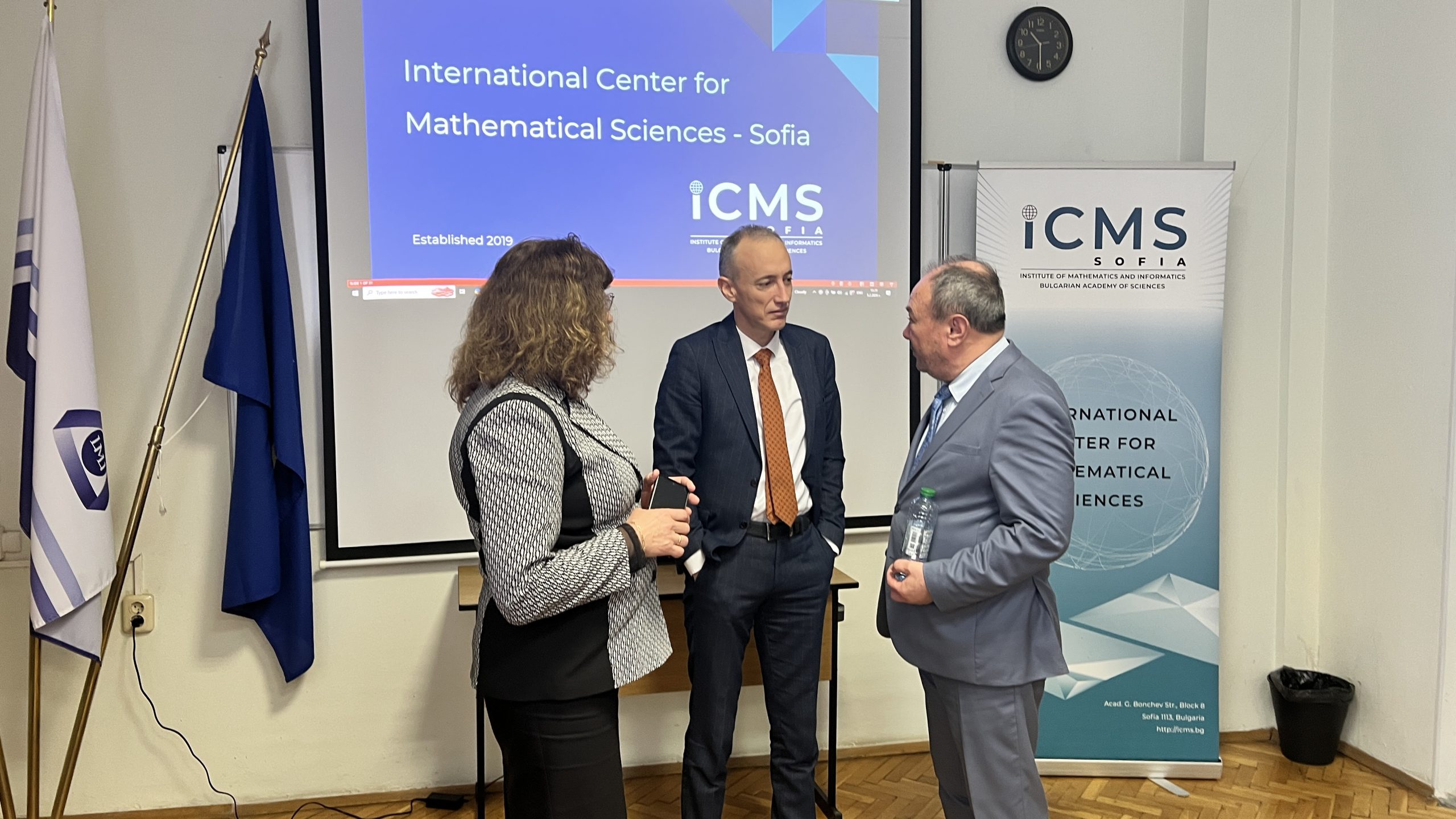
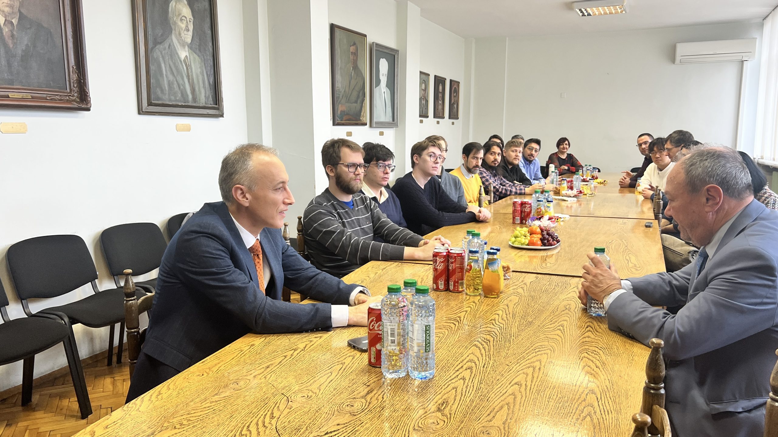
On February 5, 2026, the Minister of Education and Science Krasimir Valchev, visited the Institute of Mathematics and Informatics at the Bulgarian Academy of Sciences (IMI-BAS) to receive an overview of the development and achievements of the International Center for Mathematical Sciences (ICMS-Sofia).
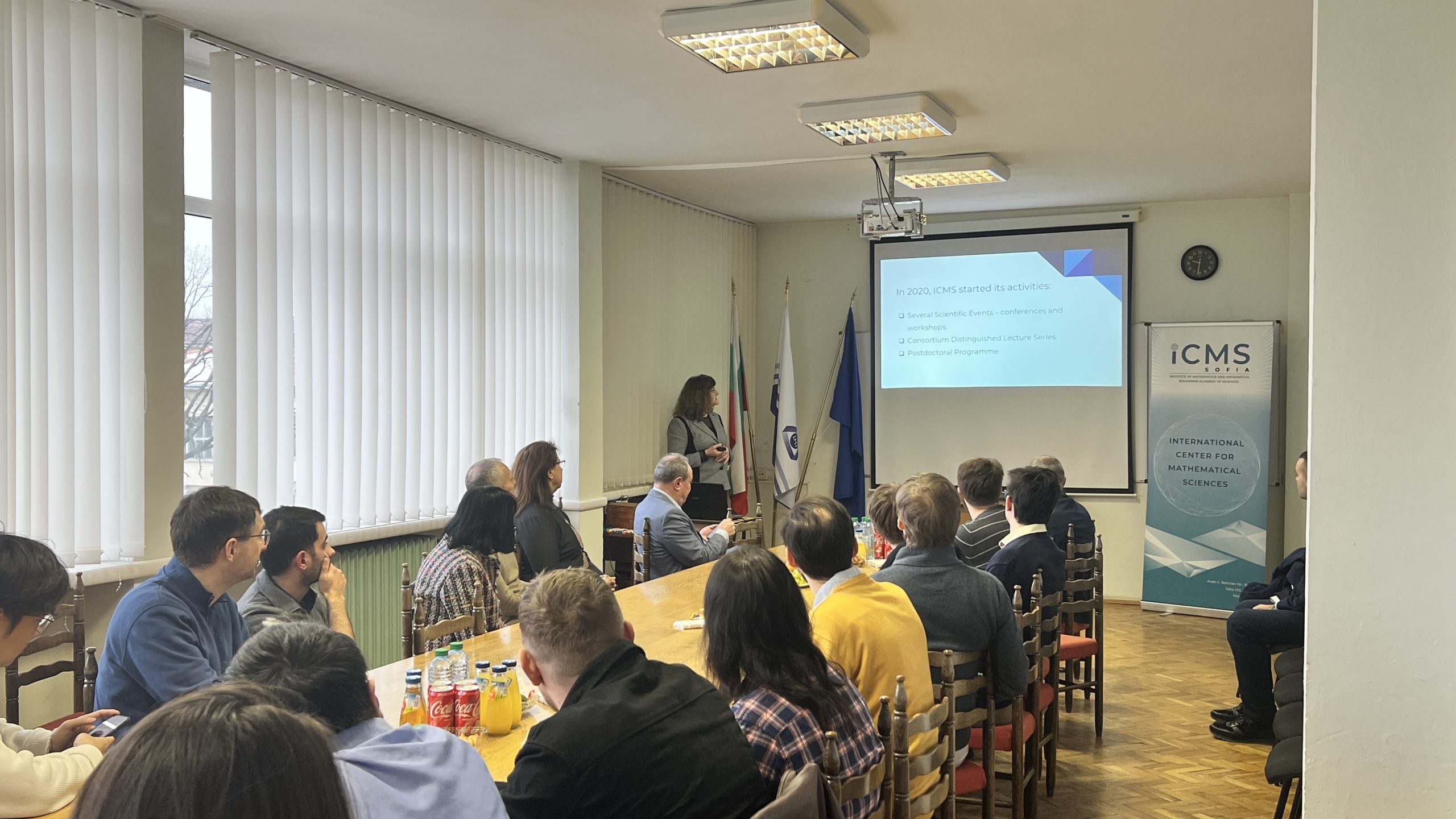
Minister Valchev was personally welcomed at IMI by Prof. Julian Revalski – Director of the International Center for Mathematical Sciences, Prof. Velichka Milousheva – Deputy Director of both IMI and ICMS-Sofia, Prof. Hristo Kostadinov – Deputy Director of IMI, and Assoc. Prof. Krassimira Ivanova – Scientific Secretary of the Institute. During the visit, the leadership presented the newly established research groups within ICMS, each led by a distinguished internationally recognized scientist in key areas of modern fundamental and applied mathematics.
Founded in 2019, the International Center for Mathematical Sciences was established as a result of the determined and visionary efforts of Prof. Blagovest Sendov, Prof. Julian Revalski, Minister Krasimir Valchev, and his deputy Karina Angelieva, as well as with the support of the Bulgarian mathematical community and diaspora. Its activities are made possible due to the financial support of the Ministry of Education and Science of the Republic of Bulgaria and Simons Foundation International, one of the most prestigious foundations for funding scientific research in the USA. Although it is only six years old, the Center has already managed to establish itself as a leading scientific organization, not only in the Balkans but far beyond.
Highlights for the 2020–2025 Period:
- Scientific Events: A total of 37 international conferences and seminars have been organized.
- Hired Researchers: 32 postdocs, 3 leading researchers, 11 established researchers, and 2 displaced scientists from Ukraine have been funded.
- Collaboration with World-renowned Scientists: five Fields Medalists have been attracted to participate in the initiatives of ICMS-Sofia: Maxim Kontsevich, Andrei Okounkov, Terence Tao, Maryna Viazovska, and Caucher Birkar.
The Center plays a particularly significant role in the global mathematical network as a member of the IMSAC (Institute of the Mathematical Sciences of the Americas Consortium). This partnership brings together institutions from Latin America, the Caribbean, Canada, the USA, and Europe for joint research projects.
The Center maintains active collaboration with the Institute of the Mathematical Sciences of the Americas (IMSA) at the University of Miami, with which ICMS has jointly carried out a successful postdoctoral program since 2021. The Center also sustains active cooperation with the French Institut des Hautes Études Scientifiques (IHÉS), a symbol of excellence in mathematics and theoretical physics.
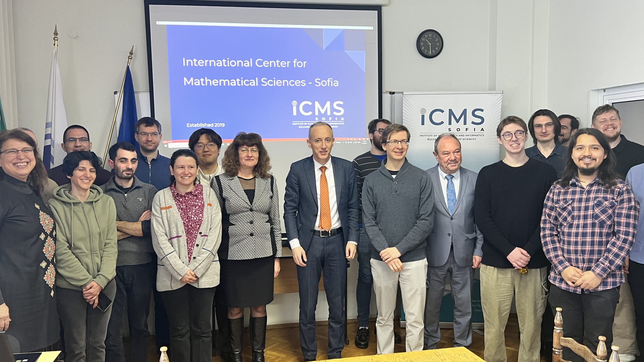
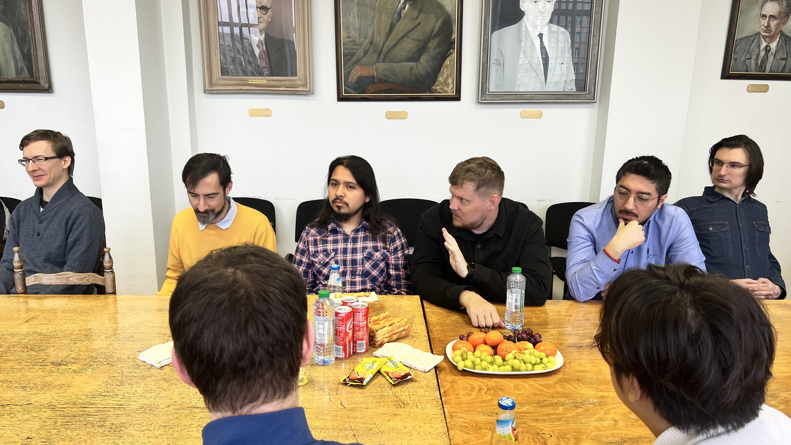
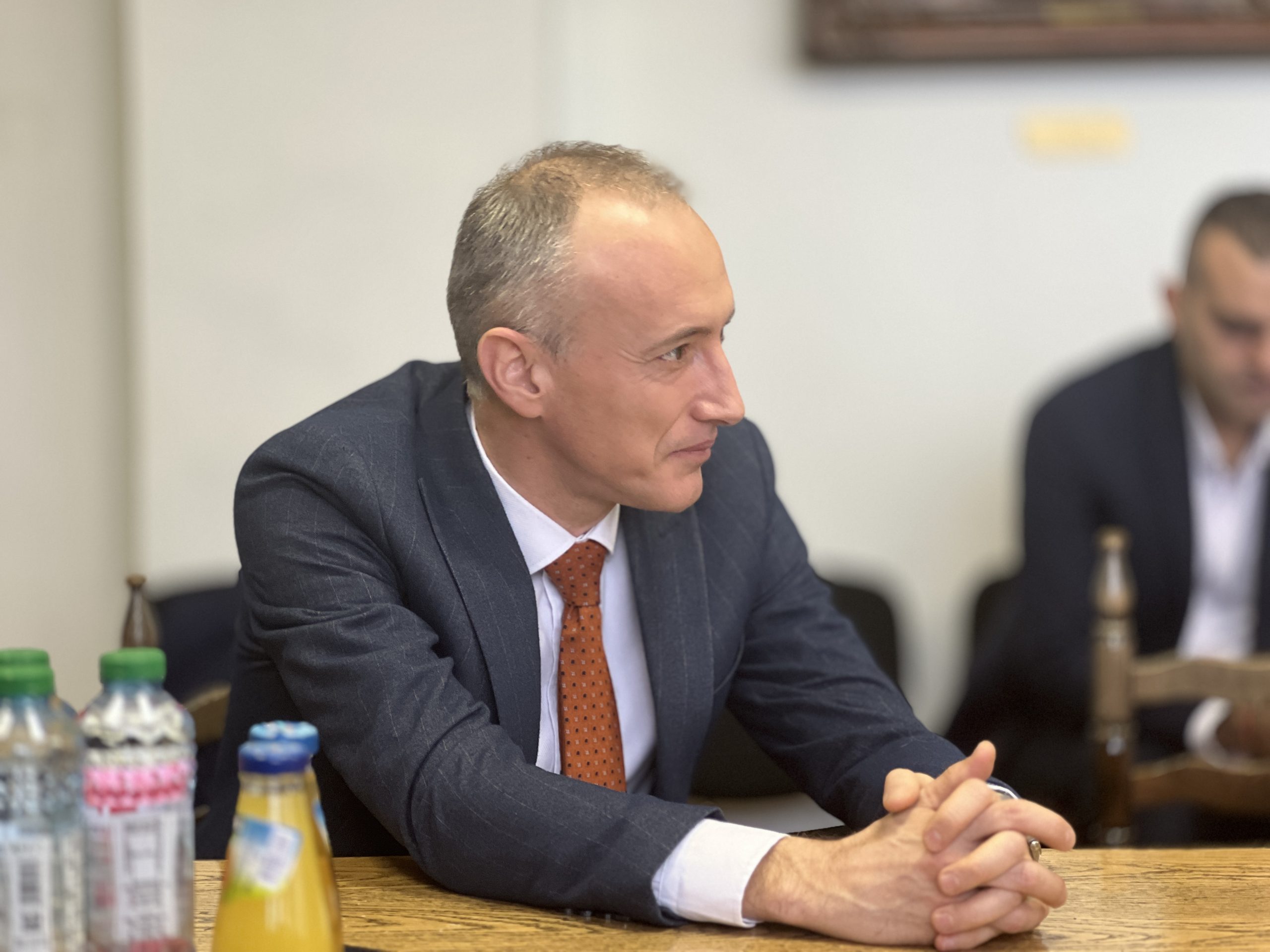
During his visit, Minister Valchev held a constructive discussion with the ICMS young researchers. He expressed his strong appreciation for the Center’s ability to attract such a large number of highly qualified international scientists who choose Bulgaria as a place for scientific development. The discussion also addressed opportunities for the sustainable advancement of mathematical research in Bulgaria and the importance of international mobility for integrating Bulgarian scientists into the global scientific community.
Administration
IMI PRIZE
IMI MATHEMATICS PRIZE
Please donate
BIC: UNCRBGSF
IBAN: BG32UNCR76303100117336
Address: Institute of Mathematics and Informatics,
Acad. G. Bonchev Str., Block 8,
1113 Sofia
VAT No.: BG000665249


Useful Links